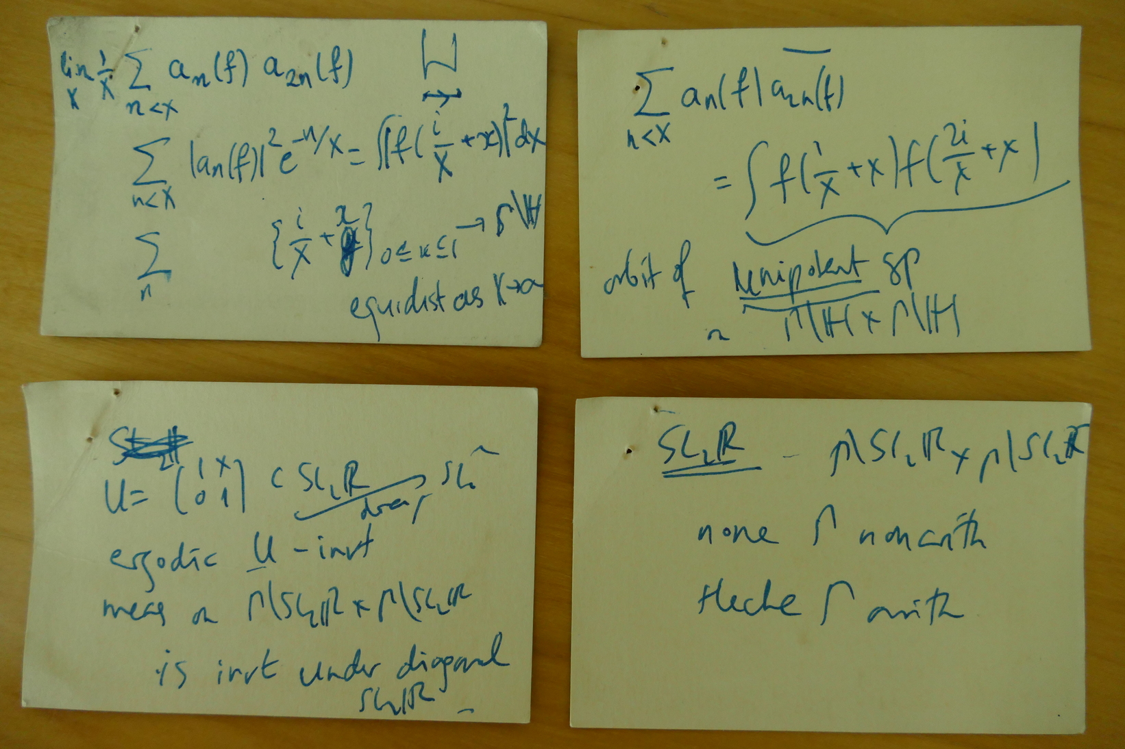
Now that Akshay Venkatesh has (deservedly) received the Fields Medal, I find myself the owner of some priceless items of mathematical history: the four restaurant cards on which, some time in (probably) 2005, Akshay sketched the argument (based on Ratner theory) that proves that the Fourier coefficients of a cusp form at 

")

\overline{a(2n)}=0.")
(Incidentally, the great persifleur of the world was also present that week in Bristol, if I remember correctly).
The story of these cards actually starts the year before in Montréal, where I participated in May in a workshop on Spectral Theory and Automorphic Forms, organized by D. Jakobson and Y. Petridis (which, incidentally, remains one of the very best, if not the best, conference that I ever attended, as the programme can suggest). There, Akshay talked about his beautiful proof (with Lindenstrauss) of the existence of cusp forms, and I remember that a few other speakers mentioned some of his ideas (one was A. Booker).
In any case, during my own lecture, I mentioned the question. The motivation is an undeservedly little known gem of analytic number theory: Duke and Iwaniec proved in 1990 that a similar non-correlation holds for Fourier coefficients of half-integral weight modular forms, a fact that is of course related to the non-existence of Hecke operators in that context. Since it is known that this non-existence is also a property of non-arithmetic groups (in fact, a characteristic one, by the arithmeticity theorem of Margulis), one should expect the non-correlation to hold also for that case. This is what Akshay told me during a later coffee break. But only during our next meeting in Bristol did he explain to me how it worked.
Note that this doesn’t quite give as much as Duke-Iwaniec: because the ergodic method only gives the existence of the limit, and no decay rate, we cannot currently (for instance) deduce a power-saving estimate for the sum of ")

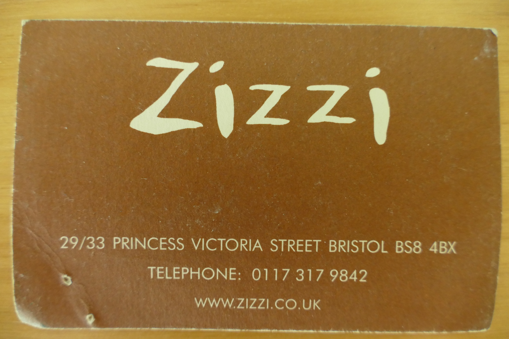
For a detailed write-up of Akshay’s argument, see this short note; if you want to go to the historic restaurant where the cards were written, here is the reverse of one of them:
If you want to make an offer for these invaluable objects, please refer to my lawyer.