[[Update (April 5, 2009): now that the Tricki is officially available, the original article below will not be updated anymore. For the latest version, see here.]]
Title: Smooth sums
Quick description: It is often difficult to evaluate asymptotically sums of the type
$latex \sum_{n=1}^N{a(n)},$
but much simpler to deal with
$latex \sum_{n\geq 1}{a(n)\varphi(n)}$
where φ is a smooth function, which vanishes or decays very fast for n larger than N. Such sums are called smoothed sums.
This trick is useful because it often turns out, either that the original problem leading to the first type of sums could be treated using the second type; or that understanding the smoothed sums may be the right path to understanding the first ones.
General discussion: The underlying facts behind this trick are two elementary properties of harmonic analysis: (1) a Fourier (or similar) transform of a product is the convolution of the Fourier transforms of the arguments; (2) in the sums above, one of the arguments in the product is an (implicit) characteristic function of the interval of summation, and Fourier transforms exchange properties of regularity with properties of decay at infinity, so that after applying the Fourier transform to the product, the smoothing function becomes a rapidly decaying factor which simplifies many further analytic manipulations. Thus, this technique may be interpreted also as some form of regularization.
The effect is the trick is thus to eliminate some purely analytic problems of convergence which are otherwise unrelated to the main issue of interest. This trick is often especially useful in situations where the other argument of the product involved is non-negative. In particular, it is very relevant for asymptotic counting problems in analytic number theory and related fields. It may also fruitfully be combined with dyadic partition arguments (see this (unwritten) tricki article).
Prerequisites: Real analysis and integration theory, complex analysis for some applications. Elementary harmonic analysis (such as Fourier transforms, or Mellin transforms, depending on the type of applications). In particular, the two facts indicated above (behavior with respect to product, and exchange of regularity and decay) are important.
Here are links to the examples to be found below:
Example 1. (Summation of Fourier series)
Example 2. (Fourier inversion formula)
Example 3. (Estimating sums of arithmetic functions)
Example 4. (The Prime Number Theorem)
Example 5. (The analytic large-sieve inequality)
Example 6. (The approximate functional equation for ζ(s))
Example 7. (The explicit formula)
——————————————————————————————–
Example 1. (Summation of Fourier series) If f is a periodic function with period 1 on the real line, which is integrable (in the Lebesgue sense, say) on the closed interval [0,1], the Fourier coefficients of f are given by
$latex a_n=\int_0^1{f(t)\exp(-2i\pi nt)dt}$
for any integer n. A basic problem of Fourier analysis is to determine when the Fourier series
$latex x\mapsto \sum_{n\in\mathbf{Z}}{a_n \exp(2i\pi n x)}$
exists and coincides with f.
Let
$latex S_N(x)=\sum_{-N\leq n\leq N}{a_n \exp(2i\pi n x)}$
be the partial sum of this series. We can also interpret the formula as
$latex S_N(x)=\sum_{n\in\mathbf{Z}}{a_n\exp(2i\pi nx)\varphi_N(x)}$
where the sum is again unbounded, but the Fourier coefficients are “twisted” with the characteristic function of the finite interval of summation
$latex \varphi_N(x)=0\ \text{if}\ |x|>N,\ \varphi_N(x)=1\ \text{if}\ |x|\leq N$
The multiplication-convolution relation of harmonic analysis and the definition of the Fourier coefficients lead to
$latex S_N(x)=\int_0^1{f(t)D_N(x-t)dt}$
where
$latex D_N(x)=\sum_{|n|\leq N}{\exp(2i\pi nx)}= \frac{\sin((2N+1)\pi x)}{\sin \pi x}$
is the so-called Dirichlet kernel of order N. This convolution expression is very useful to investigate when the partial sums converge to f(x), but it is well-known that some regularity assumptions on f are needed: there exist integrable functions f such that the Fourier series diverges almost everywhere, as first shown by Kolmogorov.
A significantly better behavior, for continuous functions f, is obtained if, instead of the partial sums above, the Fejér sums are considered:
$latex \sigma_N(x)=\sum_{-N\leq n\leq N}{a_n \exp(2i\pi n x)\left(1-\frac{|n|}{N}\right)}=\frac{1}{N}(S_0(x)+\cdots+S_{N-1}(x)).$
These are our first examples of smoothed sums, since the first expression shows that they differ from the partial sums by the replacement of the characteristic function φN(x) by the function
$latex \psi_N(x)=(1-|x|/N)\varphi_N(x)$
which is more regular: it is continuous on R. Intuitively, one may expect a better analytic behavior of those modified sums because of the averaging involved (by the second expression for the Fejér sums), or because the “smoother” cut-off at the end of the interval of summation implies that those sums should be less susceptible to sudden violent oscillations of the size of the Fourier coefficients.
This is visible analytically from the integral expression which is now
$latex \sigma_N(x)=\int_0^1{f(t)F_N(x-t)dt}$
where
$latex F_N(x)=\frac{1}{n}\frac{\sin^2(n\pi x)}{\sin^2\pi x}$
is the Fejér kernel. Because this kernel is non-negative, it is not very difficult to prove that
$latex \lim_{N\rightarrow +\infty}{\sigma_N(x)}=f(x)$
for all x if f is continuous. (And in fact, if f is of class C1, it is also easy to deduce that the original partial sum do converge, proving Dirichlet’s theorem on the convergence of Fourier series for such functions).
T. Tao mentioned in his comments that the modern version of this example, in harmonic analysis, is the theory of Littlewood-Paley multipliers, and that they are particularly important in the study of partial differential equations and the associated spaces (such as Sobolev spaces). [A reference for this will be added soon].
Example 2. (Fourier inversion formula) If we consider a function f which is integrable on R, the Fourier transform of f is the function defined by
$latex g(x)=\int_{\mathbf{R}}{f(t)\exp(-2i\pi xt)dt}$
for x in R. The Fourier inversion formula states that if g is itself integrable, then we can recover the function f by the formula
$latex f(t)=\int_{\mathbf{R}}{g(x)\exp(2i\pi xt)dx}.$
A first idea to prove this is to replace the values g(x) on the right-hand side of this expression by their definition as an integral, and apply Fubini’s theorem to exchange the two integrals; this leads formally to
$latex \int_{\mathbf{R}}{f(t)\left(\int_{\mathbf{R}}{\exp(2i\pi x(t-u)du}\right)dt}$
but the problem is that the inner integral over u does not exist in the Lebesgue sense. However, if g is replaced by a smoother version obtained by multiplying with a function φ which decays fast enough at infinity, then the same computation leads to
$latex \int_{\mathbf{R}}{g(x)\varphi(x)\exp(2i\pi xt)dx}=\int_{\mathbf{R}}{f(t)\left(\int_{\mathbf{R}}{\varphi(x)\exp(2i\pi x(t-u)du}\right)dt},$
which is now legitimate. Selecting a sequence of such functions φ which converge (pointwise) to the constant function 1, the left-hand side converges to
$latex \int_{\mathbf{R}}{g(x)\exp(2i\pi xt)dx}$
while a standard Dirac-sequence argument shows that
$latex \int_{\mathbf{R}}{\varphi(x)\exp(2i\pi xu)du}$
behaves like a Dirac function at the origin, hence the right-hand side of the smoothed formula converges to f(t).
Note. In these two first examples, one can see the “regularization” aspect very clearly, and one could also invoke more abstract ideas of the theory of distributions to express the same arguments. (For instance, for Example 2, one can say that Fourier inversion holds for the Dirac measure with Fourier transform 1, and that the formal properties involving convolution then extend the formula to more general functions). In the next examples, involving analytic number theory, it is often of the greatest importance to have explicitly quantitative estimates at all steps, and this is often more easily done using computations with functions instead of distributions. However, which functions are used for smoothing is often of little importance.
Example 3. (Estimating sums of arithmetic functions) Let a(n) be an arithmetic function, or in other words a complex-valued function defined for positive integers, and let A(x) denote the summatory function
$latex A(x)=\sum_{1\leq n\leq x}{a(n)}.$
Many different problems of analytic number theory can be expressed as the problem of understanding the asymptotic behavior of such sums as x goes to infinity. In Example 4, we describe a celebrated example, the Prime Number Theorem where a(n) is the characteristic function of the set of primes, but here we look at a slightly simpler situation where we assume that
$latex a(n)\geq 0$
and that we want to have an upper-bound for A(x), instead of an asymptotic formula. (This weakened goal might be natural, either because we do not need an asymptotic formula for further applications, or because some uniformity in parameters is needed which is easier to arrange with upper bounds). Quite often, this is approached by trying to use the properties of the Dirichlet generating series
$latex D(s)=\sum_{n\geq 1}{a(n)n^{-s}}$
provided it converges at least in some half-plane where the real part of s is larger than some C.
Then we can replace the implicit characteristic function of the interval [1,x] in A(x) by any smooth(er) function which is pointwise larger. For instance, if we choose a function φ as in the graph below
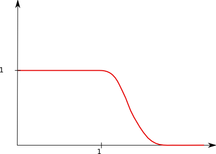
so that it is smooth, non-negative, compactly supported on [0,2], and such that
$latex \varphi(x)=1\ for\ 0\leq x\leq 1,$
then we have
$latex A(x)\leq A_{\varphi}(x)=\sum_{n\geq 1}{a(n)\varphi(n/x)}.$
Using the Mellin transform (the multiplicative counterpart to the Fourier transform), we can write
$latex \varphi(y)=\frac{1}{2i\pi}\int_{\sigma-i\infty}^{\sigma+i\infty}{\hat{\varphi}(s)y^{-s}ds}$
where we integrate over a vertical line in the complex plane with real part σ>0, and
$latex \hat{\varphi}(s)=\int_0^{+\infty}{\varphi(x)x^{s-1}dx}.$
Because we use a compactly supported function, it is easy to justify the exchange of the sum over n and the integral representing φ(n/x), and obtain
$latex A(x)\leq \frac{1}{2i\pi}\int_{\sigma-i\infty}^{\sigma+i\infty}{\hat{\varphi}(s)x^sD(s)ds}.$
Now we are free to use any technique of complex analysis to try to estimate this integral. The usual idea is to move the line of integration (using Cauchy’s theorem) as far to the left as possible (since the modulus of xs diminishes when the real part of s does). For this, clearly, one needs to know how far D(s) can be analytically continued, but it is equally important to have some control of the integrand high along vertical lines to justify the change of line of integration, and this depends on the decay properties of the Mellin transform at infinity, which amount exactly to the regularity properties of φ itself. If φ was the characteristic function of the interval [1,x], then the Mellin transform only decays like 1/s for s high in a vertical strip, and multiplying this with any functions D(s) which does not tend to 0 leads, at best, to conditionally convergent integrals. On the other hand, if φ is compactly supported on [0,+∞[, it is very easy to check that the Mellin transform is not only holomorphic when the real part of s is positive (which allows changing the contour of integration that far), but also it decaysfaster than any polynomial in vertical strips, so that any D(s) which has at most polynomial growth in vertical strips can be involved in this manipulation.
(A prototype of this, though it doesn’t involve a compactly supported function, is φ(x)=e-x, for which we have
$latex \hat{\varphi}(s)=\Gamma(s),$
the Gamma function, which decays exponentially fast in vertical strips by the complex Stirling formula: we have
$latex |\Gamma(\sigma+it)|\leq C|t|^{\sigma-1/2}\exp(-\pi|t|/2)$
for some constant C, uniformly for σ in any bounded interval and |t|>1).
Finally, even if an asymptotic formula for A(x) is desired, it may be much easier to prove them by using upper and lower bounds
$latex A_1(x)\leq A(x)\leq A_2(x)$
where
$latex A_i(x)=\sum_{n\geq 1}{a(n)\varphi_i(n)}$
and the smoothing functions, this time, have graphs as described below
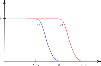
with a parameter y<x which is left free to optimize later on. In a concrete case, one may (for instance) prove — using the smoothness of the sums — that
$latex A_1(x)=x-y+O(x^{2/3}),\ \ \ \ \ A_2(x)=x+y+O(x^{2/3})$
and then the choice of y=x2/3 and the encadrement above imply that
$latex A(x)=x+O(x^{2/3}).$
An example of this is found in the “circle” problem of Gauss, which asks the best possible estimate for the number of points with integral coordinates inside a disc with increasing radius. Gauss himself, by a simple square-packing argument proved that
$latex |\{(n,m)\ |\ n,m\geq 1,\ n^2+m^2\leq x\}|=\frac{\pi}{4}x+O(x^{1/2})$
(where the error term can also be interpreted as the approximate length of the boundary circle). The first improvement of the error term is due to Voronoi:
$latex |\{(n,m)\ |\ n,m\geq 1,\ n^2+m^2\leq x\}|=\frac{\pi}{4}x+O(x^{1/3})$
and it is typically proved by smoothing techniques. (Though there are also arguments involving the Euler-Maclaurin formula).
Note also that, in smoothed form, a much better error term can easily be achieved, for instance
$latex \sum_{m\leq x}{r(m)(1-m/x)}=\frac{\pi}{8}x+O(x^{-1/4}).$
Example 4. (The Prime Number Theorem) The first proofs of the Prime Number Theorem
$latex |\{p\leq x\ |\ p\text{ is prime}\}|\sim \frac{x}{\log x}$
as x goes to infinity, due (independently) to J. Hadamard and C.J. de la Vallée Poussin in 1896, were implementations of the previous example, either with a(n) the characteristic function of the primes, or
$latex a(p)=\log p\ \ \ \text{if } p \text{ is prime},\ \ \ \ a(n)=0\text{ otherwise}$
(which leads to slightly simpler formulas, as already discovered by Chebychev when working with elementary methods). Both proofs used smoothing in a somewhat implicit form. Hadamard’s proof, for instance, amounted roughly to considering
$latex B(x)=\sum_{n\leq x}{a(n)\log (x/n)}$
(where the smoothing is present because the function which is inserted is zero at the end of the summation), and rewriting it as
$latex B(x)=\frac{1}{2i\pi}\int_{3-i\infty}^{3+i\infty}{-\frac{\zeta^{\prime}(s)}{\zeta(s)}x^s\frac{ds}{s^2}}$
where the point is that the smoothing in B(x) is the reason for the appearance of the factor s-2, which itself allows the integral to converge absolutely, even after shifting the integration to a contour close to but to the left of the line where the real part of s is 1. Hadamard adds (see the last page) a remark that, in so doing, he avoids the well-deserved criticisms levelled by de la Vallée Poussin against those arguments which, being based on A(x) itself, involve an integral with merely a factor s-1, which do not converge absolutely.
The last step of the proof is then an easy argument, using the fact that A(x) is increasing, that shows that the asymptotic formula for B(x) implies the expected asymptotic formula for A(x), i.e., the Prime Number Theorem.
There is nothing special about suing this particular form of smoothing; almost any kind would work here.
Note that, in sharp contrast with the circle problem mentioned in Example 3, it is not possible to use smoothing here to diminish too much the error term in the counting function: because there are infinitely many zeros of the Riemann zeta function on the critical line, the best possible result is of the type
$latex \sum_{p}{(\log p)\varphi(p/x)}=\text{(Main term)}+ O(sqrt{x}),$
and this would follow from the Riemann Hypothesis.
Note. It is of course the case that the proof of the Prime Number Theorem involves much more than this trick of smoothing! However, it is clearly the case that trying to dispense with it — as can be done — means spending a lot of energy dealing with purely analytic issues of convergence and exchange of sums and integrals, which become completely obvious after smoothing.
Example 5. (The analytic large-sieve inequality) Sometimes smoothing can be used efficiently for estimating sums involving oscillating terms (like exponential sums), although no direct comparison holds as it does in Example 3. As an example, consider the dual analytic large sieve inequality
$latex \sum_{n=1}^N{\left|\sum_{r=1}^R{a(r)\exp(2i\pi n\xi_r)}\right|^2}\leq \Delta \sum_{r=1}^N{|a(r)|^2}$
which can be proved to hold with
$latex \Delta=N-1+\delta^{-1}$
for all N, alll complex coefficients a(r), provided the real numbers ξr are δ-spaced modulo 1, i.e., we have
$latex \min_{m\in\mathbf{Z}}{|m+\xi_r-\xi_s|}\geq \delta$
if r is distinct from s.
To prove this inequality one is tempted to open the square on the left-hand side, and bring sum over n inside to obtain
$latex \sum_{r,s}{a(r)\overline{a(s)}W(r,s)}$
with
$latex W(r,s)=\sum_{n=1}^N{\exp(2i\pi (\xi_r-\xi_s)n)}.$
This is a geometric sum, and is easily summed, but it is not so easy to get a good grip on it afterwards in summing over r and s. Although Montgomery and Vaughan succeeded, it is instructive to note that a much quicker argument — though with a weaker result — can be obtained by smoothing W(r,s). However, after opening the square, it is not clear how to insert a smoothing factor without (maybe) changing the sums completely — since the coefficients a(r) are arbitrary. So one must insert the smoothing beforehand: the left-hand side of the inequality is non-negative and can be bounded by
$latex \sum_{n=1}^N{\left|\sum_{r=1}^R{a(r)\exp(2i\pi n\xi_r)}\right|^2}\varphi(n/N)$
for any smooth function φ which is equal to 1 on [1,N]. This leads to modified sums
$latex W_{\varphi}(r,s)=\sum_{n=1}^N{\exp(2i\pi (\xi_r-\xi_s)n)\varphi(n/N)}$
which can be evaluated and transformed, for instance, by Poisson’s formula to exploit the rapid decay of the Fourier transform of φ.
The best functions for this particular example (leading to the inequality with N-1+1/δ) are remarkable analytic functions studied by Beurling and later Selberg. This illustrates that whereas the particular smoothing function used is often irrelevant, it may be of great importance and subtlety for specific applications.
Example 6. (The “approximate functional equation”) This next example shows how to use smoothing to represent an analytic function given by a Dirichlet series outside of the region of absolute convergence, so that it can be analyzed further. As an example, the series
$latex L(s)=1-\frac{1}{3^s}+\frac{1}{5^s}-\cdots=\sum_{n\geq 1}{\frac{(-1)^{n+1}}{(2n-1)^s}}$
converges absolutely only when the real part of s is larger than 1 (it converges conditionally when the real part is positive). It is known to have analytic continuation to an entire function, but in order to investigate its properties in the critical strip, say when the real part of s is 1/2, it is necessary to find some convenient alternative expression valid in this region. [Note that what is explained below applies also to the Riemann zeta function, with a small complication in presentation due to the presence of a pole at s=1; this is why we describe the case of L(s).]
So assume s has real part between 0 and 1. A common procedure is to pick a non-negative smooth function φ on [0,+∞[, with compact support or rapide decay, equal to one on a neighborhood of 0, and with
$latex \int_0^{+\infty}{\varphi(t)dt}=1$
and then consider, for a parameter X>1, the smoothed sum
$latex S(X)=\sum_{n\geq 1}{\frac{(-1)^{n-1}}{(2n-1)^s}\varphi(n/X)}$
which makes sense for all s if φ decays fast enough. The role of X is, intuitively, as the effective length of the sum.
Using Mellin inversion as in Example 3, we get
$latex S(X)=\frac{1}{2i\pi}\int_{3-i\infty}^{3+i\infty}{L(s+w)\hat{\varphi}(w)X^wds}.$
Now shift the vertical line of integration to the left; because L(s) has at most polynomial growth vertical strips (a non-obvious fact, but one that can be proved without requiring much specific information because of the general Phragmen-Lindelöf principle) and because the Mellin transform of the smooth function φ decays faster than any polynomial, this shift is easy to justify.
Now where do we get poles while performing this shift? The recipe for φ (specifically, that it equals 1 close to 0 and has integral 1) easily imply that φ(w) has a simple pole at w=0 with residue 1, and this leads to a contribution equal to
$latex L(s)X^0\hat{\varphi}(0)=L(s),$
so that
$latex S(X)=L(s)+R(X)$
where the remainder R(X), if we shifted the intregration to the line with real part c is
$latex R(X)=\frac{1}{2i\pi}\int_{c-i\infty}^{c+i\infty}{L(s+w)\hat{\varphi}(w)X^wds}.$
This can be estimated fairly easily if c is very negative, but one can also use the functional equation of L(s) to express R(X) as a sum very similar to S(X), except that s is replaced with 1-s, and the new sum has effective length roughly equal to (|t|+1)/X, where t is the imaginary part of s (the smoothing function is also different). Thus one gets, roughly, an expression for L(s) as the sum of two sums of lengths, the products of which is equal to |t|+1. This is a very general fact in the study of L-functions and of the basic tools for the study of their analytic properties.
Example 7. (The “explicit formula” of prime number theory) In his paper on the Riemann zeta function, Riemann stated that the function π(x) which counts primes up to x is given by
$latex \pi(x)=\mathrm{Li}(x)+\sum_{\rho}{\mathrm{Li}(x^{\rho})}+\text{(other elementary terms)}$
where the sum runs over zeros of ζ(s). This “explicit formula” and similar ones can be very useful to understand many aspects of the distribution of primes, but this particular one is hard to justify for convergence reasons. However, provided one looks at a smoothed sum
$latex \sum_{p}{(\log p)\varphi(p/x)}$
(which has effective length x), it is a simple exercise in contour integration to obtain an explicit formula which converges very well, involving a sum over the zeros of the zeta function weighted with the Mellin (or Laplace, or Fourier) transform of φ.
Generalizations of it to primes in arithmetic progressions or Dirichlet L-functions are very efficient, for instance, in finding very strong estimates — assuming the Generalized Riemann Hypothesis — for the smallest prime in an arithmetic progression, or similar problems.
—————————————————————————————–
References: The technique of smoothing is not usually discussed in detail in textbooks. One exception is in my introductory book on analytic number theory (in French, so smooth sums are called sommes lisses or sommes lissées): see Section 2.3 in particular where the technique is introduced; it is then used throughout the book quite systematically even when — sometimes — it could be dispensed with.
For details of Examples 4, 5, 6, 7, 8, one can look in my book with Henryk Iwaniec (see Chapters 5 and 7 in particular), although the technique is used there without particular comments.
Kowalski, you are a retarded cunt. Didn’t you know that? Well, now you know! How retarded one should be in order to refresh a cache for comments pages once per hour while comments feed is updated immediately? Apparently, as retarded as Kowalski is.
Now about those smooth sums. I tell you what, Kowalsi! You can shove those fucking smooth sums into your fucking asshole, and enjoy the smoothing they provide to your fucking shit, you dumb fuck!
Kowalski, you are a retarded cunt. Didn’t you know that? Well, now you know! How retarded one should be in order to refresh a cache for comments pages once per hour while comments feed is updated immediately? Apparently, as retarded as Kowalski is.
Now about those smooth sums. I tell you what, Kowalski! You can shove those fucking smooth sums into your fucking asshole, and enjoy the smoothing they provide to your fucking shit, you dumb fuck!