Page 32 – E. Kowalski's blog

La dure loi du sport (or, one point one way, one point another way)

The world cup of the world’s greatest team sport has just ended with the final victory of the New Zealand team against the XV de France. Although it is somewhat bitter to fail for the third time in the final, all partisans of the French artistry on the field (where viril, mais correct is but one of the noble guiding principles) recognize that a victory — and it was rather close! — would have been undeserved. Indeed, the French qualified for the final only after a rather lucky win against a brilliant Welsh team in the semi-final. After fighting more than an hour with one man less, the Welsh barely lost by one point (9 to 8, and more importantly, without the French scoring a single try). I feel that the French’s loss by the same point (7 to 8) is fair. Their tremendous fighting spirit shows that their presence here today was not, in fact, entirely undeserved, but a win would have left a sour taste in my mouth. Let’s hope that in four years, they will (for once…) actually play throughout the tournament with the same intensity. And then let the best team win…

Trevisan’s L^1-style Cheeger inequality

My expander class at ETH continues, and for the moment the course notes are kept updated (and in fact I have some more in the notes than I did in class).

Last week, I presented the inequalities relating the definition of expanders based on the expansion ratio with the “spectral” definition. In fact, I used the random walk definition first, which is only very slightly different for general families of graphs (with bounded valency), and is entirely equivalent for regular graphs. For a connected $k$ -regular graph $\Gamma$ , the inequalities state that
$\frac{2}{k}\lambda_1(\Gamma)\leq h(\Gamma)\leq k\sqrt{2\lambda_1(\Gamma)},$
where:

$\lambda_1(\Gamma)$ is the smallest non-zero eigenvalue of the normalized Laplace operator $\Delta$ , i.e., the operator acting on functions on the vertex set by
$\Delta\varphi(x)=\varphi(x)-\frac{1}{k}\sum_{y\text{ adjacent to x}}{\varphi(y)}$ .
$h(\Gamma)$ is the expansion ratio of $\Gamma$ , given by $h(\Gamma)=\min_{1\leq |W|\leq |\Gamma|/2}\frac{|E(W)|}{|W|},$ the set $E(W)$ in the numerator being the set of edges in $\Gamma$ with one extremity in $W$ and one outside.

The left-hand inequality is rather simple, once one knows (or notices) the variational characterization
$\lambda_1(\Gamma)=\min_{\varphi\perp 1}\frac{\langle \Delta\varphi,\varphi\rangle}{\|\varphi\|^2}$
of the spectral gap: basically, for a characteristic function $\varphi$ of a set $W$ of vertices, the right-hand side of this expression reduces (almost) to the corresponding ratio $|E(W)|/|W|$ . The second inequality, which is called the discrete Cheeger inequality, is rather more subtle.

The proof I presented is the one presented by L. Trevisan in his recent lectures on expanders (see, specifically, Lecture 4). Here, the idea is to construct a test set for $h(\Gamma)$ of the form
$W_t=\{x\in V_{\Gamma}\,\mid\, \varphi(x)\leq t\},$
for a suitable real-valued function $\varphi$ on the group. The only minor difference is that, in order to motivate the distribution of a random “threshold” $t$ that Trevisan uses to construct those test sets, I first stated a general lemma where the threshold is picked according to a fairly general probability measure. Then I first showed what happens for a uniform choice in this interval, to motivate the “better” one that leads to Cheeger’s inequality.

As it turns out, I just found an older blog post of Trevisan explaining his proof, where he also discusses first the computations based on the uniform measure supported on $[\min \varphi,\max\varphi]$ , and explains why it is problematic.

But there is some good in this inequality. First, the precise form it takes (which I didn’t find elsewhere, and will therefore name Trevisan’s inequality) is
$h(\Gamma)\leq \frac{A}{B}$
where, for any non-constant real-valued function $\varphi$ with minimum $a$ , maximum $b$ and median $t_0$ , we have
$A=\frac{1}{2}\sum_{x,y\in V}{a(x,y)|\varphi(x)-\varphi(y)|},$
(where $a(x,y)$ is the number of edges between $x$ and $y$ ) and
$B=\sum_{x\in V}{|\varphi(x)-t_0|}.$

The interesting fact is that this can be sharper than Cheeger’s inequality. Indeed, this happens at least for the family of graphs $\Gamma_n$ which are the Cayley graphs of $\mathfrak{S}_n$ with respect to the generating set
$S_n=\{(1\ 2),(1\ 2\ \cdots\ n)^{\pm 1}\}.$
From an analysis of the random walks by Diaconis and Saloff-Coste (see Example 1 in Section 3 of their paper), it is known that
$\lambda_1(\Gamma_n)\asymp \frac{1}{n^3},$
and Cheeger’s inequality leads to
$h(\Gamma_n)\ll n^{-3/2}.$
However (unless I completely messed up my computations…), one sees that the test function used by Diaconis and Saloff-Coste, namely the cyclic distance between $\sigma^{-1}(1)$ and $\sigma^{-1}(2)$ , satisfies
$\frac{A}{B}\ll \frac{1}{n^2},$
and therefore we get a better upper-bound
$h(\Gamma)\ll \frac{1}{n^2}$
using Trevisan’s inequality.

(Incidentally, we see here an easy example of a sequence of graphs which forms an esperantist family, but is not an expander.)

Inkscape and LaTeX

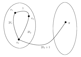
I’m a great fan of the open-source vector-drawing software Inkscape. Although I don’t have that many figures in my papers (or notes), I’ve found it quite accessible and easy to use to produce high-quality results. And just yesterday, as I wanted to add a picture to my notes on expander graphs, I learnt of a very nice new feature: from version 0.48 onward, one can select a special option when saving a drawing as PDF that creates an auxiliary LaTeX file, which can then be incorporated in the source file (using the standard \input command) and which contains (and processes) all the text found in the drawing. This makes it very easy to add arbitrary LaTeX (math) formulas with Inkscape.

For example, the SVG file

produces a PDF file

and a LaTeX file, and when the latter is inserted, the document reveals the beautiful picture

In the “never too late to learn that” section…

As a number theorist interested in probability, I have accumulated my knowledge of that field (such as it is…) in a rather haphazard fashion, as is probably (pun intended) typical. The gaps in my understanding are wide and not really far between, and I can’t generally expect to take advantage of teaching a class to fill them (we have very good probabilists in Zürich), though I did teach introductory probability two years in Bordeaux. So it’s not so surprising that I stumbled this morning in my lecture on expanders when defining a Markov chain (which deserves some “tsk, tsk” from my ancestors, since my mathematical genealogy does trace back to Markov…)

More precisely, given a graph $\Gamma$ , say $k$ -regular, I defined a random walk on $\Gamma$ as a sequence $(X_n)$ of random variables taking values in the vertex set $V$ , and which satisfy the conditional probability identity
$\mathbf{P}(X_{n+1}=y\mid X_n=x)=\frac{a(x,y)}{k}$
for all $n\geq 0$ , and all vertices $x, y$ , where $a(x,y)$ is the number of edges (unoriented, oeuf corse) between $x$ and $y$ .

But, as one of the CS people attending the lecture pointed out, this is wrong! The definition of a Markov chain requires that be able to condition further back in the past: for any choices of $x_0, x_1,\ldots, x_n$ , one asks that
$\mathbf{P}(X_{n+1}=y\mid X_0=x_0,\ldots, X_n=x_n)=\mathbf{P}(X_{n+1}=y\mid X_n=x)=\frac{a(x,y)}{k}$
which corresponds to the intuition that the behavior at time $n$ be independent of the part trajectory of the walk, except of course for the actual value at time $n$ .

What puzzled me no end was that I had failed to notice the problem, simply because this more general condition did not play any role in what I was doing, namely in proving the convergence to equilibrium of the random walk! The difference, which was clarified by my colleague M. Einsiedler, is that although the “wrong” definition allows you to compute uniquely the distribution of each step $X_n$ as a function of the initial distribution $X_0$ , and of the transition probabilities $a(x,y)/k$ , one needs the actual Markov condition in order to compute the joint distribution of the whole process $(X_n)$ , i.e., in order to express such probabilities as
$\mathbf{P}(X_n=x_n,\ldots,X_n=x_0)$
as functions of the distribution of $X_0$ and the transition probabilities.

(My confusion arose partly from the fact that, up to this class, I exclusively used random walks on groups as Markov chains, defined using independent steps, and these are automatically Markovian; I’ve actually exploited the “strong” Markov property in a recent paper with F. Jouve and D. Zywina, but in that specialized context, the point above — I’m not sure if it deserves to be called “subtle!” — didn’t register…)

Action graphs

The beginning of my lecture notes on expander graphs is now available. These first sections are really elementary. If it were not grossly insulting to the noble brotherhood (and sisterhood) of bookkeepers, I would say that I deal here mostly with bookkeeping: setting up a rigorous “coding” of the class of graphs I want to consider (which are unoriented graphs where multiple edges are allowed as well as loops), defining maps between such graphs, and setting up the basic examples of Cayley graphs and Schreier graphs.

But still, I managed to trip once on the last point, and my first definition turned out to be rather bad. Of course, it is not that I don’t know what a Schreier graph is supposed to be, but rather that I stumbled when expressing properly this intuition in the specific “category” I am using (where a graph is a triple $(V,E,e)$ , with vertex set $V$ , edge set $E$ , and
$e\,:\, E\rightarrow \{\text{subsets of } V\text{ with } 1 \text{ or } 2\text{ elements}\}$
is the “endpoints” map.)

What I knew about the Schreier graph of a group $G$ with respect to a subgroup $H$ and a (symmetric) generating set $S$ is that it should be $|S|$ -regular, and the combinatorial Laplace operator $\Delta$ should be given by
$\Delta\varphi(x)=\varphi(x)-\frac{1}{|S|}\sum_{s\in S}{\varphi(sx)},$
for any function $\varphi$ on $G/H$ . This I managed to ensure on the second try, though the definition is a bit more complicated than I would like.

I actually wrote things down for more general “action graphs”, which are pretty much the obvious thing: given an action of the group $G$ on a set $X$ , one takes $X$ as vertices, and moves along edges (set up properly) from $x$ to $s\cdot x$ for $s$ in the given subset $S$ of $G$ . Here is a query concerning this: do these general graphs have a standard name? I have not seem the definition in this generality before, but it seems very natural and should be something well-known, hence named. (Of course, using decomposition in orbits, such a graph is a disjoint union of Schreier graphs modulo stabilizers of certain points of $X$ , but that doesn’t make it less natural.)

In any case, here is an illustration of the action graph for the symmetric group $S_5$ , with generators $S=\{(1\ 2), (1\ 2\ 3\ 4\ 5), (1\ 5\ 4\ 3\ 2)\}$ , acting on $X=\{1,2,3,4,5\}$ by evaluation:

Equivalently, this is the Schreier graph of $G/H$ with respect to $S$ , where $H$ is the stabilizer of $1$ .

As it should be, this graph is $3$ -regular, and this property would fail if loops and multiple edges were not permitted. It is true that, in that case, the resulting graph (a cycle of length $5$ ) would remain regular after removing loops and multiple edges, but the interested reader will have no problem checking that if $S$ is replaced by
$S'=S\cup\{(1\ 2\ 3), (1\ 3\ 2)\},$
removing loops and multiple edges from the corresponding action graph leads to a non-regular graph. (The vertex 1 has three neighbors then, namely $\{2, 3, 5\}$ , while the others have only 2.)

(The typesetting of the graph is done using the tkz-graph package already mentioned in my previous post.)